Maps: U.S. climate trends

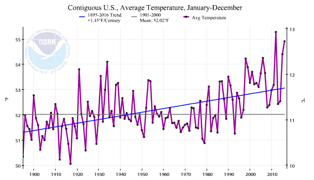
Our climate is changing and one of the most straightforward ways to understand these changes is by examining linear trends. In climate, to determine the linear trend we plot data values by when they occurred in the past and then determining a “best fit” line through that data. The slope of the line gives us the trend. Using this method we know that the since 1895 the contiguous U.S. temperature has warmed at rate of 1.45 °F per century.

However, temperatures are not warming uniformly in space or time. The cold parts of the day (nights), cold parts of the year (winter), and cold parts of the world (high latitudes) tend to be warming the fastest. To help our users understand how different times and places are warming at different rates, NCEI has created trend maps for the contiguous U.S. of average temperature, minimum temperature (nighttime lows), maximum temperature (afternoon highs), and precipitation for the annual period and each month and season. The maps are created in a method similar to the linear trend analysis described above, but for each grid box in NCEI’s nClimgrid 5km gridded dataset. This Beyond the Data post will explore these new maps and explain some of the findings when we spatially examine trends across the Lower 48.

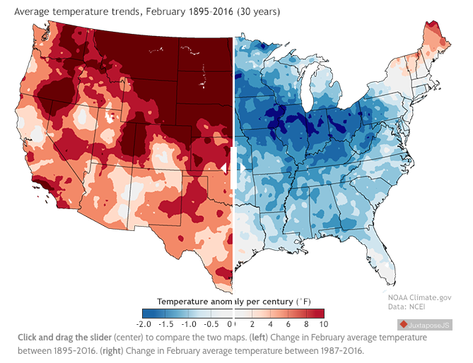
The curious case of February

In addition to creating trend maps for the different temperature and precipitation variables, we also produce trends maps for two different periods of record – the last 30 years (1987-2016) and the entire period of record (1895-2016). Depending on what a user might be interested in understanding, they might find utility in one or both of the time periods. For example, an electric power company might be interested in recent changes in temperature, while an ecologist trying to understand changes in migratory patterns might be more interested in the entire period of record.

...